Feedback induced patterns in bistable networks

Effects of feedbacks on self-organization phenomena in networks of diffusively coupled bistable elements are investigated. For regular trees, an approximate analytical theory for localized stationary patterns under application of global feedbacks is constructed. Using it, properties of such patterns in different parts of the parameter space are discussed. Numerical investigations are performed for large random Erdös-Rényi and scale-free networks. In both kinds of systems, localized stationary activation patterns have been observed. The active nodes in such a pattern form a subnetwork, whose size decreases as the feedback intensity is increased. For strong feedbacks, active subnetworks are organized as trees. Additionally, local feedbacks affecting only the nodes with high degrees (i.e. hubs) or the periphery nodes are considered.

An one-component network-organized bistable system, generally reads

\[
\dot{u}_i = f(u_i) + D\left( \sum_{j=1}^{N}\!T_{ij}u_j – \sum_{j=1}^{N}\!T_{ji}u_i \right)\,\]
where \(u\) is the local activator density, function \(f(u_i,h)=u_i(h-u_i)(u_i-a)\) specifies local bistable dynamics and \(D\) is the coupling strength. \(\mathbf{T}\) is the adjacency matrix that describes the connectivity structure of the network; its elements are \(T_{ij}=1\), if there is a link connecting the nodes \(i\) and \(j\) (\(i,j=1,…,N\)), and \(T_{ij}=0\) otherwise. Processes in undirected networks, where the adjacency matrix \(\mathbf{T}\) is symmetric (\(T_{ij} = T_{ji}\)),
\[
\dot{u}_i = f(u_i) + D \sum_{j=1}^{N}\!T_{ij}\left(u_j – u_i \right)\,\]

We introduce the global feedback through the parameter \(h\), i.e. as
\[h = h_0 + \mu(S-S_0)\,,\]
where \(\mu>0\) is the intensity of the feedback, \(S=\sum_{j=1}^{N}\!u_j\,\) is the total activation of the network and \(S_0\) is a parameter defining the size of localized patterns. In our simulations, it was taken equal to the number of the nodes which were initially activated. Hence, the threshold \(h\) depends now on the total activation; it increases when more nodes are activated, so that a negative feedback is realized.

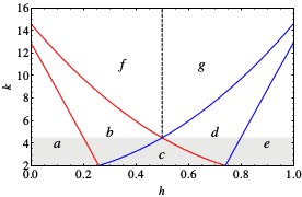
Bistable trees

In the figure below we see a regular tree with the branching factor \(k-1\), where \(k\) is the nodes degree.

In such a tree, all nodes, lying at the same distance \(l\) from the origin, can be grouped into a single shell (see figure above). The tree can then be treated as a chain of \(l = 1,2,3,\ldots\) asymmetrically coupled shells. Suppose that we have taken a node which belongs to the shell \(l\). This node should be diffusively coupled to \(k-1\) nodes in the next shell \(l+1\) and to just one node in the previous shell \(l-1\). Introducing the activation level \(u_l\) in the shell \(l\), the evolution of the activator can therefore be described by the equation

\[
\dot{u}_{l} = f(u_{l}) + D (u_{l-1}-u_{l}) + D(k-1)(u_{l+1}-u_{l})\,.
\]

This latter equation can be analysed (see [1,2]) and reveal all dynamical behaviour that summarized in the next bifurcation diagram in the \(h-k\) parameter space.

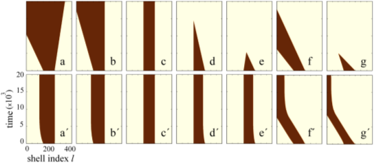
Space-time plots in the next figure show all possible evolution of an initial activation in presence \((a-g)\) and absence \((a’-g’)\) of negative feedback for the corresponding parameter regimes.

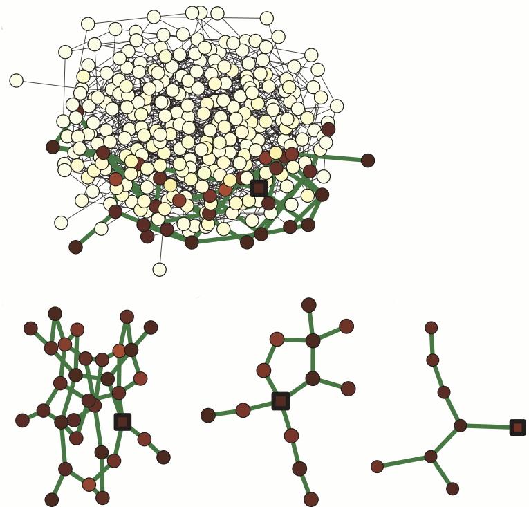
Random bistable networks

Global negative feedback

As we see in the next figure, the activation that is applied to one node (marked by a square) starts to spread out. This produced a growing cluster of activated nodes. Its growth is however accompanied by an increase of the negative feedback. Consequently, the threshold \(h\) increases with the size of the cluster, making the activation more difficult. As a result, the growth of the activated cluster is slowed down and finally stopps. Thus, a stationary activation pattern, representing a small subnetwork embedded in the entire network (see three examples in the same figure) became formed.

Local negative feedback

So far, we have assumed that the negative feedback was global. However, it is also possible that the feedback acts only on a subset of nodes. Suppose for example that the parameters \(h_i\), which control the dynamics of individual nodes \(i\), have different sensitivity to the global control signal depending on the degrees of such nodes,

\[h_i = h_0 + \mu B(k_i)(S-S_0)\,,\]
where \(B(k_i)\) is the step function, \(B(k)=1\) if \(k\lt k_0\) and \(B(k)=0\) otherwise.

In this case, the negative feedback is applied only to the periphery nodes with small degrees \(k\), where \(k\lt k_0\). By introducing such local feedback, we can control directly the dynamics of periphery nodes, whereas hubs remain non-affected and have a constant threshold \(h=h_0\) sufficient for activation spreading. The simulations show that, in this situation, the activation applied to a hub node starts to spread forming a cluster of activated nodes with high degrees \(k\geq k_0\), whose further growth to the periphery nodes is suppressed by the feedback. Thus, an active stationary cluster, localized on the hubs, becomes formed.
Alternatively, the step function \(B(k)=1\) if \(k\gt k_0\) and \(B(k)=0\) otherwise, induced a localized pattern of active peripheral nodes only (see figure below).

Further reading:

1. N. E. Kouvaris, H. Kori and A. S. Mikhailov:
   Traveling and pinned fronts in bistable reaction-diffusion systems on networks.
   PLoS ONE 7(9): e45029 (2012).
   [PLoS ONE]
2. N. E. Kouvaris and A. S. Mikhailov:
   Feedback-induced stationary localized patterns in networks of diffusively coupled bistable elements.
   EPL (Europhysics Letters) 102, 16003 (2013).
   [EPL] [arXiv]