Two-state exitable systems

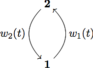
A two-state unit is considered as an abstract modification for an excitable system. Each state is characterized by a different waiting time distribution. This non-Markovian approach allows for a renewal process description of the system dynamics. Exact formulas for the interspike interval distribution and power spectral density are found. In the limit of an infinity ensemble of globally coupled units the mean-field equations for the populations of both states are derived. Depending on the coupling strength and on the noise intensity the ensemble undergoes saddle-node bifurcations and demonstrates bistability, while a pitchfork bifurcation emerges on a cusp point. The ensemble undergoes Hopf bifurcations and bulk oscillations emerge, in the onset of coherent activation events, only when the feedback affects individual units with a certain time delay.

Single excitable unit

The transition to oscillatory behaviour from excitable or bistable dynamics is one of the fundamental bifurcations in complex systems. It is a well studied mechanism for single excitable units and for neuronal ensembles. There is a various number of neuron models with two or three components including activator and inhibitor dynamics. They describe the voltage and the gating dynamics determining the rest, activation and refractory states of a neuron. Here we propose an abstract neuron model which constitutes a semi-Markovian process for a single unit that changes between two states according to a discrete time Markov chain. However, it spends in each state a random amount of time, distributed by the density functions \(w_1(t)\) and \(w_2(t)\), respectively.

Although the process is not Markovian, the waiting time in a certain state is independent of the time spent in the preceding state. This single unit aims to mimic a single stochastic excitable system when specific distributions are used. Hence, the transition \(1\to 2\) holds for the activation events while the transition \(2\to 1\) models the return to the rest state. The transition \(1\to 2\) is modeled as a rate process:\[w_{1}(t) = \gamma\exp(-\gamma t)\]where both mean and variance equals \(1/\gamma\). This is the escape time needed, for an excitable system, to leave the rest state, under the influence of noise. The transition \(2\to 1\) is modeled by an Erlang distribution:\[w_2(t) = \frac{\alpha_2}{t_2\Gamma(\alpha_2)}
\left(\frac{\alpha_2 t}{t_2}\right)^{\alpha_2 – 1}
\exp\left(-\frac{\alpha_2 t}{t_2}\right)\]
where \(\alpha_2\) is integer. The mean value equals \(t_2\) and the variance \(t_2^2/\alpha_2\). This distribution describes the waiting time in the excited state corresponding to the quasi-deterministic spike production when the impact of fluctuations is negligible. Therefore the width of \(w_2\) has to be narrow, realized by choosing large values of \(\alpha_2\) where the Erlang distribution is close to a \(\delta\)-distribution. The choice of \(w_1\) and \(w_2\) results from the basic features of excitable systems, which have a stable fixed point. By noise, they can escape from that fixed point with a certain randomly distributed time, modeled by \(w_1\). The following excursion in phase space is less affected by noise, however the time can also vary with a small dispersion. This motivates us to the assumption for our model that the resting state corresponds to the fixed point and the excited state to the excursion in the phase space.

Coupled excitable units

Coupled excitable units with time delay

Further reading:

1. N. Kouvaris, F. Müller and L. Schimansky-Geier:
   Ensembles of excitable two-state units with delayed feedback.
   Phys. Rev. E 82, 061124 (2010)
   [PRE]
2. N. Kouvaris, L. Schimansky-Geier and E. Schöll:
   Control of coherence in excitable systems by the interplay of noise and time-delay.
   Eur. Phys. J. Special Topics 191, 29-51 (2010)
   [EPJ-ST]